
Why batch optimization matters
Bayesian optimization is widely used for expensive black-box problems: situations where each trial is costly, the search space is large, and there is no simple formula telling us where the optimum lies [1][2]. In these settings, the method uses past observations to make a more informed decision about what to try next.
In the simplest setup, the process is sequential. One candidate is selected, evaluated, and then the model is updated before the next decision is made. This works well when experiments must be run one at a time.
However, many practical workflows are parallel rather than purely sequential. A lab may be able to prepare multiple samples in the same round, a compute cluster may run many jobs at once, or a customer may prefer to receive several recommendations in a single cycle. The literature on batch and parallel Bayesian optimization was developed precisely to address this mismatch between a sequential decision rule and a parallel experimental reality [2-7].
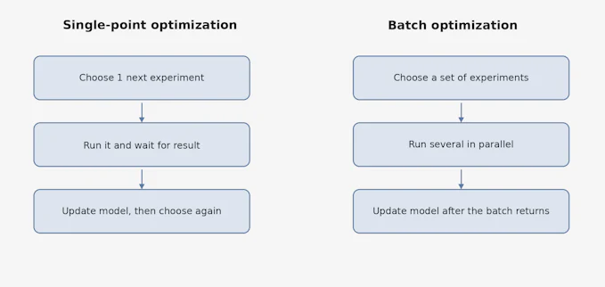
Figure 1. A simple comparison between single-point optimization and batch optimization. In batch optimization, the key challenge is not only choosing good candidates, but choosing candidates that make sense together as one experimental round.
A brief intuitive view of Bayesian optimization
A simple way to explain Bayesian optimization is to imagine a researcher exploring an unfamiliar landscape. The researcher wants to find a good region quickly, but each experiment is expensive. Instead of trying everything, the researcher uses the data already collected to estimate where success is more likely and where uncertainty is still high.
This is why many introductions describe Bayesian optimization as balancing two goals: focusing on promising areas and still exploring uncertain areas [1]. For this article, the important point is not the mathematics behind that balance, but the practical consequence: the method is meant to help us spend a limited experimental budget more wisely.
What changes when we choose a batch
Once several experiments can be run in parallel, the decision problem changes. We are no longer asking only, “What is the next best point?” Instead, we are asking, “What is the next best set of points?”
That difference matters because the value of a batch is not simply the sum of individual scores. If the top five recommended candidates are all minor variations of one another, the batch may consume a lot of resource while teaching us very little new. A useful batch therefore needs two things at once: good individual promise and reasonable diversity within the batch.
This issue appears throughout the batch Bayesian optimization literature. Researchers propose different ways to account for the interactions among points that are chosen together, because once one point is selected, later points in the same batch should not ignore that choice [3-7].
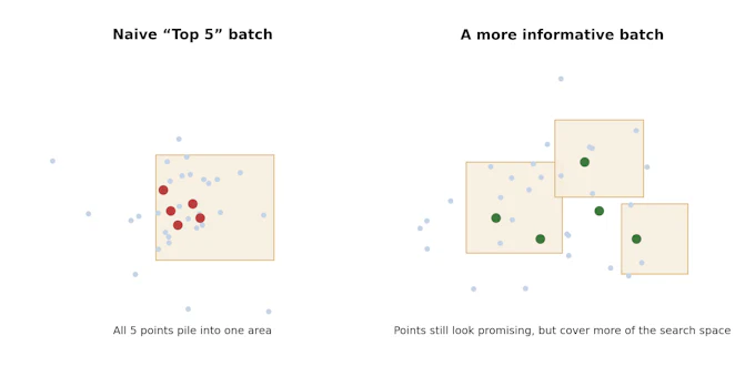
Figure 2. Why a batch is not just “the top five points.” The left panel shows a wasteful batch in which all selected points crowd into one local area. The right panel shows a more informative batch: still promising, but less redundant.
Main families of batch strategies
The literature contains many variants, but for a non-specialist audience it is helpful to group them into a few broad families.
Sequential simulation approaches
One common idea is to build the batch one point at a time. After the first candidate is selected, the algorithm temporarily pretends that some information about that candidate is already known. It then uses that temporary assumption to choose the second candidate, and repeats the process until the batch is full. Constant Liar belongs to this family [3][4].
Diversity-promoting approaches
Another family tries to reduce redundancy more directly. A representative example is local penalization, which discourages later points in the same batch from clustering too closely around earlier points. The goal is not diversity for its own sake, but a better spread across regions that still look useful [5].
Joint batch scoring approaches
A more direct but often more demanding idea is to score the whole batch together rather than constructing it greedily. Multi-point expected improvement, often written as q-EI, is a well-known example. It is attractive because it matches the true batch problem more closely, but several papers note that optimizing such criteria can become computationally challenging as the batch grows [6].
Sampling-based parallel approaches
Another line of work uses sampling-based rules such as parallel Thompson sampling. These methods can be conceptually simple and naturally compatible with parallel execution, especially when evaluation times are variable or asynchronous execution matters [7].
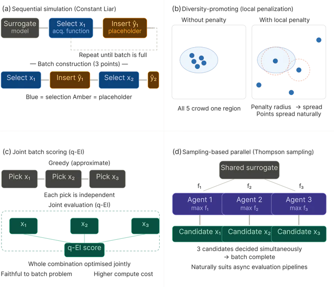
Figure 3. Overview of four representative batch Bayesian optimisation strategies.
(a) Sequential simulation builds the batch greedily using placeholder values.
(b) Diversity-promoting penalises clustering. (c) Joint scoring evaluates the whole batch together.
(d) Sampling-based methods draw independent posterior samples in parallel.
Constant Liar
Constant Liar is one of the best-known practical heuristics for building a batch in a step-by-step way. Its core idea is straightforward. After choosing the first candidate, the algorithm does not wait for the real result. Instead, it inserts a temporary placeholder value for that point, updates the model as if that value were already observed, and then picks the next candidate [3][4].
The name comes from the fact that the placeholder is not the real result. It is a deliberately invented stand-in. In the original line of work on parallel Kriging-based optimization, this family of heuristics was introduced as a way to avoid the intractability of exact batch calculations while still accounting for earlier choices in the same batch [3].
This gives Constant Liar a very practical interpretation: it is a structured approximation that makes sequential logic usable in a batch setting.

Figure 4. Constant Liar as a workflow. The method greedily builds a batch by inserting a temporary value for each newly selected point so that the next choice is not made in complete ignorance of the earlier ones.
Why Constant Liar is still used
In this article, we present Constant Liar as a representative practical strategy for batch optimization, rather than as a universally preferred solution.
Even so, there are clear reasons why teams still use it. First, it is relatively easy to understand and explain. Second, it extends a familiar sequential workflow into a batch workflow without requiring a complete redesign. Third, the literature repeatedly treats it as a useful baseline or benchmark because it is simple, practical, and often effective enough for real experimental pipelines [4][6].
In our internal evaluations, Constant Liar was not uniformly the best-performing method in every scenario. Nevertheless, it showed consistently stable optimization behavior across a broad range of settings, including both low- and high-dimensional problems, different numbers of objectives, discrete and continuous parameter spaces, and functions with both smooth and steep response characteristics. This breadth of applicability is one of its key practical strengths. Even when another method outperforms it in a particular setting, Constant Liar tends to remain a reliable choice across diverse optimization conditions.
In other words, Constant Liar survives not because it is guaranteed to be universally best, but because it often offers a good engineering trade-off between simplicity, cost, and performance.
Where other methods may be preferable
Constant Liar is still an approximation. Its behavior depends on the placeholder value used during batch construction, and different choices can push the algorithm toward more conservative or more aggressive behavior [4].
If a team needs a method that accounts for the whole batch more directly, q-EI-based methods may be more attractive, although the computational cost can be higher [6]. If avoiding point clustering is the primary concern, diversity-oriented methods such as local penalization may be appealing [5]. If the workflow is highly asynchronous, sampling-based parallel methods can be especially attractive [7].
The larger lesson is that batch optimization is a family of design choices, not a single fixed recipe.
Key takeaway
Batch optimization in Bayesian optimization is about making better use of each experimental round when several experiments can be run in parallel. The problem is not only to find good candidates, but to find a good group of candidates. Constant Liar is a classic example of how practitioners approximate that group decision in a simple and workable way, and the wider batch optimization literature shows why different workflows may prefer different strategies [1-7].
Appendix: A quick comparison of representative batch strategy families
Strategy family | Simple intuition | Main strength | Typical trade-off |
|---|---|---|---|
Sequential simulation (e.g., Constant Liar) | Pretend earlier batch points already have temporary results, then keep selecting | Easy to explain and implement | Uses an approximation, not the true outcomes |
Diversity-promoting (e.g., local penalization) | Push later selections away from earlier ones | Reduces redundancy within a batch | Can spread points too widely if overdone |
Joint batch scoring (e.g., q-EI) | Score the value of the whole batch together | Closer to the true batch decision | Can be more computationally demanding |
Sampling-based parallel methods (e.g., parallel TS) | Use randomized posterior-guided choices in parallel | Works naturally with parallel and asynchronous settings | Behavior may be less straightforward to explain to non-specialists |
References
- Brochu, E., Cora, V. M., & de Freitas, N. (2010). A Tutorial on Bayesian Optimization of Expensive Cost Functions, with Application to Active User Modeling and Hierarchical Reinforcement Learning. arXiv:1012.2599. https://arxiv.org/abs/1012.2599
- Snoek, J., Larochelle, H., & Adams, R. P. (2012). Practical Bayesian Optimization of Machine Learning Algorithms. Advances in Neural Information Processing Systems 25. https://proceedings.neurips.cc/paper/2012/file/05311655a15b75fab86956663e1819cd-Paper.pdf
- Ginsbourger, D., Le Riche, R., & Carraro, L. (2008/2010). Kriging is Well-Suited to Parallelize Optimization / A Multi-points Criterion for Deterministic Parallel Global Optimization based on Gaussian Processes. Introduces Constant Liar and related heuristics for parallel EI-style selection. https://www.cs.ubc.ca/labs/algorithms/EARG/stack/2010_CI_Ginsbourger-ParallelKriging.pdf
- Azimi, J., Fern, A., & Fern, X. (2012). Hybrid Batch Bayesian Optimization. ICML 2012. Discusses Constant Liar as a representative batch heuristic and analyzes simulated sequential batch policies. https://icml.cc/2012/papers/614.pdf
- González, J., Dai, Z., Lawrence, N. D., & Hennig, P. (2016). Batch Bayesian Optimization via Local Penalization. AISTATS 2016. https://proceedings.mlr.press/v51/gonzalez16a.html
- Wang, J., Clark, S. C., Liu, E., & Frazier, P. I. (2020). Parallel Bayesian Global Optimization of Expensive Functions. Operations Research, 68(2), 1-21. Compares q-EI-style optimization with Constant Liar baselines and discusses computational trade-offs. https://pubsonline.informs.org/doi/10.1287/opre.2019.1966
- Kandasamy, K., Krishnamurthy, A., Schneider, J., & Póczos, B. (2018). Parallelised Bayesian Optimisation via Thompson Sampling. AISTATS 2018. https://proceedings.mlr.press/v84/kandasamy18a.html